Kernel Goodness-of-Fit Testing¶

Figuring out the origin of a particular set of data is difficult. However, insights gained from the origin of a set of samples (i.e., its target density function) can be instrumental in understanding its characteristics. This sort of testing is desirable in practice to answer questions such as: does this sample correctly represent this population? Can a certain statistical phenomena be attributed to a given distribution?

For anyone interested in questions like the above, this module of the package is perfect! The goal of goodness-of-fit testing is to determine, given a set of samples, how likely it is that these were generated from a target density function. The tests can be found in hyppo.kgof, and will be elaborated upon in detail below. But let's take a look at some of the mathematical theory behind the test formation:

Consider a known probability density \(p\) and a sample \(\{ \mathbf{x}_i \}_{i=1}^n \sim q\) where \(q\) is an unknown density, a goodness-of-fit test proposes null and alternative hypotheses:

\[\begin{split}H_0 &: p = q \\ H_1 &: p \neq q\end{split}\]

In other words, the GoF test tests whether or not the sample \(\{ \mathbf{x}_i \}_{i=1}^n\) is distributed according to a known \(p\).

The implemented test relies on a new test statistic called The Finite-Set Stein Discrepancy (FSSD) which is a discrepancy measure between a density and a sample. Unique features of the new goodness-of-fit test are:

It makes only a few mild assumptions on the distributions \(p\) and \(q\). The model \(p\) can take almost any form. The normalizer of \(p\) is not assumed known. The test only assesses the goodness of \(p\) through \(\nabla_{\mathbf{x}} \log p(\mathbf{x})\) i.e., the first derivative of the log density.

It returns a set of points (features) which indicate where \(p\) fails to fit the data.

A simple Gaussian model¶

Assume that \(p(\mathbf{x}) = \mathcal{N}(\mathbf{0}, \mathbf{I})\) in \(\mathbb{R}^2\) (two-dimensional space). The data \(\{ \mathbf{x}_i \}_{i=1}^n \sim q = \mathcal{N}([m, 0], \mathbf{I})\) where \(m\) specifies the mean of the first coordinate of \(q\). From this setting, if \(m\neq 0\), then \(H_1\) is true and the test should reject \(H_0\). First construct the log density function for the model

from hyppo.kgof import DataSource
from hyppo.kgof import KGauss
from hyppo.kgof import IsotropicNormal
from hyppo.kgof import fit_gaussian_draw, meddistance
from hyppo.kgof import FSSD, FSSDH0SimCovObs
import matplotlib.pyplot as plt
import autograd.numpy as np
from numpy.random import default_rng


def isogauss_log_den(X):
    mean = np.zeros(2)
    variance = 1
    unden = -np.sum((X - mean) ** 2, 1) / (2.0 * variance)
    return unden

This function computes the log of an unnormalized density. This works fine as this test only requires a \(\nabla_{\mathbf{x}} \log p(\mathbf{x})\) which does not depend on the normalizer. The gradient \(\nabla_{\mathbf{x}} \log p(\mathbf{x})\) will be automatically computed by autograd. In this kgof package, a model \(p\) can be specified by implementing the class hyppo.kgof.density.UnnormalizedDensity. Implementing this directly is a bit tedious, however. Construct an UnnormalizedDensity which will represent a Gaussian model. All the implemented goodness-of-fit tests take this object as input.

# Next, draw a sample from q.
# Drawing n points from q
m = 1  # If m = 0, p = q and H_0 is true

seed = 4
rng = default_rng(seed)
n = 400
X = rng.standard_normal(size=(n, 2)) + np.array([m, 0])

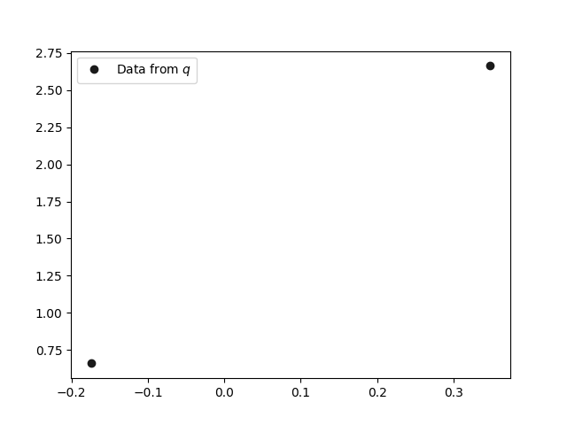
# Plot the data from q
plt.plot(X[0], X[1], "ko", label="Data from $q$")
plt.legend()

Out:

<matplotlib.legend.Legend object at 0x7f34f124c700>

Conduct an FSSD kernel goodness-of-fit test for an isotropic normal density with mean 0 and variance 1.

mean = 0
variance = 1

J = 1
sig2 = meddistance(X, subsample=1000) ** 2
k = KGauss(sig2)
isonorm = IsotropicNormal(mean, variance)

# random test locations
V = fit_gaussian_draw(X, J, seed=seed + 1)
null_sim = FSSDH0SimCovObs(n_simulate=200, seed=3)
fssd = FSSD(isonorm, k, V, null_sim=null_sim, alpha=0.01)

tresult = fssd.test(X, return_simulated_stats=True)
tresult

Out:

{'alpha': 0.01, 'pvalue': 0.0, 'test_stat': 61.381677133523624, 'h0_rejected': True, 'n_simulate': 200, 'sim_stats': array([ 1.29505800e+00,  1.67265325e+00, -4.18928718e-01, -3.64716821e-01,
       -1.66912847e-02, -3.78038231e-01,  1.33200407e+00, -3.98921406e-01,
       -2.36446579e-01,  3.33737208e+00, -4.64725554e-01, -3.37015925e-01,
       -4.36473061e-01, -2.87369594e-01, -1.11727056e-01, -4.31770142e-01,
       -4.03145994e-01, -4.57998703e-01, -7.44147383e-02, -4.63554465e-01,
        2.22045414e-01,  3.05893270e-01, -1.63648321e-01, -2.05162124e-01,
       -2.22886917e-01,  1.99801693e-01,  7.50023033e-01, -4.55847208e-01,
       -2.94006289e-01, -1.08927388e-01, -1.91444199e-01,  2.68226671e-02,
       -2.15590297e-01, -3.68241357e-01, -4.77671202e-01, -1.01386077e-01,
        2.20128025e+00, -5.65522585e-02,  2.22251002e-02,  4.98466945e-01,
       -4.56088783e-01, -2.71785863e-01,  5.09249847e-02, -9.52141224e-02,
       -3.24696751e-01, -3.85619288e-01,  1.66764497e-01,  5.12673650e-01,
       -4.64942679e-01, -7.41002043e-02, -4.27616323e-01, -2.00556482e-01,
        4.30640231e-01, -3.27291492e-01, -3.81744200e-01, -2.77085515e-01,
       -4.05516204e-01,  1.77222357e+00,  1.55483407e-01, -4.00649402e-01,
        3.99503323e-01, -3.46333243e-01, -9.51284301e-02, -2.44963435e-01,
        1.02569807e+00, -1.20333150e-01, -9.18755875e-02,  3.53207530e-02,
        1.04636792e+00, -2.93014248e-01, -3.92598286e-01, -3.58798299e-01,
        4.29386847e-01,  2.38064745e-01, -4.32440186e-01, -1.01889703e-01,
        2.46123845e-01,  7.42347011e-02, -4.29859309e-01,  4.88036562e-01,
        4.49016616e-01, -6.58828872e-02,  2.23891137e-01, -3.66162811e-02,
       -2.23273732e-01, -2.46187351e-01,  6.93625947e-02, -2.27892939e-01,
        1.80305185e-01,  2.24201439e-01, -2.89680224e-03, -3.99045246e-01,
        4.82730410e-02, -2.50519730e-01,  5.53768270e-01,  5.01135293e-01,
       -3.29829270e-01,  1.47994165e-03,  4.79506926e-01, -4.16410683e-01,
       -4.43601823e-01, -2.49985297e-01, -1.83200527e-01, -2.42339812e-01,
       -2.10089675e-01, -3.34655743e-02, -4.06077458e-01, -2.71197716e-01,
       -4.31046678e-01,  1.78652885e+00,  6.14092989e-01,  2.53231974e-01,
        1.07948538e+00, -1.83321893e-01, -3.60491633e-01, -2.69505724e-01,
        1.23361889e+00,  1.66775735e-02, -7.82649304e-02,  8.81528203e-02,
       -1.33695940e-01, -2.55178423e-01, -2.24438405e-01,  3.32585666e-02,
        9.30002885e-01, -2.80485753e-01, -1.47310632e-01, -4.04904267e-01,
        5.36137942e-01,  1.00611770e+00,  2.64646242e-01, -3.92722014e-02,
       -3.76839233e-01, -2.45222426e-01,  3.33546562e-01, -1.53041562e-01,
       -3.59049475e-01,  1.02519151e+00, -3.07988174e-01, -2.61996855e-01,
        1.42060258e-01, -3.41159793e-01,  1.72388757e+00, -9.31083735e-02,
       -2.02661986e-01, -2.56374011e-02,  4.26360487e-01, -3.89692165e-01,
       -2.43593901e-01, -4.80521194e-01, -3.37468468e-01, -3.77529682e-01,
       -4.18442631e-01,  3.33532401e-01,  4.24536272e-01, -4.60648590e-01,
       -1.52007122e-01, -3.24335590e-01, -2.37672071e-01, -4.32792136e-01,
       -2.40598408e-01, -2.17722823e-01, -4.07966557e-01, -2.63541636e-01,
        6.57109691e-01,  5.82972698e-01,  1.31551202e+00, -1.69689492e-01,
       -3.30063454e-01, -2.47830312e-01, -2.00079223e-01, -9.21681332e-02,
        8.92569825e-02, -4.05677281e-01,  3.78614538e-01, -3.68343164e-01,
       -4.12283836e-01,  1.92626781e-01, -3.56523266e-01,  1.05245873e+00,
       -9.97929834e-02,  1.08046121e+00, -3.68377347e-01, -4.22860454e-01,
       -2.94034806e-01, -2.53152802e-01, -8.97622283e-02, -3.32802455e-01,
       -4.81461428e-01,  9.35869869e-01, -3.24303391e-01, -2.71013811e-02,
       -3.42021417e-01, -1.31627480e-01, -2.82334270e-01,  5.02914336e-03,
       -3.38396516e-01,  1.52447279e-01, -4.69440071e-01, -3.16895302e-01])}

Total running time of the script: ( 0 minutes 0.086 seconds)

Gallery generated by Sphinx-Gallery

Conditional Independence Testing

Benchmarks