Note
Click here to download the full example code
Independence Testing
Finding trends in data is pretty hard. Independence testing is a fundamental tool that helps us find trends in data and make further decisions based on these results. This testing is desirable to answer many question such as: does brain connectivity effect creativity? Does gene expression effect cancer? Does something effect something else?
If you are interested in questions of this mold, this module of the package is for you!
All our tests can be found in hyppo.independence, and will be elaborated in
detail below. But before that, let's look at the mathematical formulations:
Consider random variables \(X\) and \(Y\) with distributions \(F_X\) and \(F_Y\) respectively, and joint distribution is \(F_{XY} = F_{Y|X} F_X\). When performing independence testing, we are seeing whether or not \(F_{Y|X} = F_Y\). That is, we are testing
Like all the other tests within hyppo, each method has a statistic and
test method. The test method is the one that returns the test statistic
and p-values, among other outputs, and is the one that is used most often in the
examples, tutorials, etc.
The p-value returned is calculated using a permutation test using
hyppo.tools.perm_test unless otherwise specified.
Specifics about how the test statistics are calculated for each in
hyppo.independence can be found in the docstring of the respective test. Here,
we overview subsets of the types of independence tests we offer in hyppo, and special
parameters unique to those tests.
Now, let's look at unique properties of some of the tests in hyppo.independence:
Cannonical correlation (CCA) and Rank value (RV)
Cannonical correlation (CCA) and Rank value (RV) are multivariate analogues
of Pearson's correlation.
More details can be found in hyppo.independence.CCA and
hyppo.independence.RV.
The following applies to both:
Note
- Pros
Very fast
Similar to tests found in scientific literature
- Cons
Not accurate when compared to other tests in most situations
Makes dangerous variance assumptions about the data, among others (similar assumptions to Pearson's correlation)
Neither of these test are distance based, and so do not have a compute_distance
parameter.
Otherwise, these tests runs like any other test.
Heller Heller Gorfine (HHG)
A number of tests within hyppo.independence use the concept of inter-sample
distance, or kernel similarity, to generate powerful indpendence tests.
Heller Heller Gorfine (HHG) is a powerful multivariate independence test that
compares intersample distance, and computes a Pearson statistic.
More details can be found in hyppo.independence.HHG.
Note
- Pros
Very accurate in certain settings
Has fast implementation
- Cons
Very slow (computationally complex)
Test statistic not very interpretable, not between (-1, 1)
This test runs like any other test and can be implemented as below:
import timeit

import numpy as np

setup_code = """
from hyppo.independence import HHG
from hyppo.tools import w_shaped
x, y = w_shaped(n=100, p=3, noise=True)
"""

t_hhg = timeit.Timer(stmt="HHG().test(x, y, auto=False)", setup=setup_code)
t_fast_hhg = timeit.Timer(stmt="HHG().test(x, y, auto=True)", setup=setup_code)

hhg_time = np.array(t_hhg.timeit(number=1))  # original HHG
fast_hhg_time = np.array(t_fast_hhg.timeit(number=5)) / 5  # fast HHG

print("Original HHG time: {0:.3g}s".format(hhg_time))
print("Fast HHG time: {0:.3g}s".format(fast_hhg_time))
Out:
Original HHG time: 6.21s
Fast HHG time: 0.382s
Distance Correlation (Dcorr) and Hilbert Schmidt Independence Criterion (Hsic)
Distance Correlation (Dcorr) is a powerful multivariate independence test based on
energy distance.
Hilbert Schmidt Independence Criterion (Hsic) is a kernel-based analogue to Dcorr
that uses the a Gaussian median kernel by default [1].
More details can be found in hyppo.independence.Dcorr and
hyppo.independence.Hsic.
The following applies to both:
Note
- Pros
Accurate, powerful independence test for multivariate and nonlinear data
Has enticing empiral properties (foundation of some of the other tests in the package)
Has fast implementations (fastest test in the package)
- Cons
Slightly less accurate as the above tests
For Hsic, kernels are used instead of distances with the compute_kernel parameter.
Any addition, if the bias variant of the test statistic is required, then the bias
parameter can be set to True. In general, we do not recommend doing this.
Otherwise, these tests runs like any other test.
Since Dcorr and Hsic are implemented similarly, let's look at Dcorr.
import timeit

import numpy as np

setup_code = """
from hyppo.independence import Dcorr
from hyppo.tools import w_shaped
x1, y1 = w_shaped(n=100, p=3, noise=True)
x2, y2 = w_shaped(n=100, p=1, noise=True)
"""

t_perm = timeit.Timer(stmt="Dcorr().test(x1, y1, auto=False)", setup=setup_code)
t_chisq = timeit.Timer(stmt="Dcorr().test(x1, y1, auto=True)", setup=setup_code)
t_fast_perm = timeit.Timer(stmt="Dcorr().test(x2, y2, auto=True)", setup=setup_code)
t_fast_chisq = timeit.Timer(stmt="Dcorr().test(x2, y2, auto=True)", setup=setup_code)

perm_time = np.array(t_perm.timeit(number=1))  # permutation Dcorr
chisq_time = np.array(t_chisq.timeit(number=1000)) / 1000  # fast Dcorr
fast_perm_time = np.array(t_fast_perm.timeit(number=1))  # permutation Dcorr
fast_chisq_time = np.array(t_fast_chisq.timeit(number=1000)) / 1000  # fast Dcorr

print("Permutation time: {0:.3g}s".format(perm_time))
print("Fast time (chi-square): {0:.3g}s".format(chisq_time))
print("Permutation time (fast statistic): {0:.3g}s".format(fast_perm_time))
print("Fast time (fast statistic chi-square): {0:.3g}s".format(fast_chisq_time))
Out:
Permutation time: 0.314s
Fast time (chi-square): 0.000465s
Permutation time (fast statistic): 0.000564s
Fast time (fast statistic chi-square): 0.000455s
Look at the time increases when using the fast test!
The fast test approximates the null distribution as a chi-squared random variable,
and so is far faster than the permutation method.
To call it, simply set auto to True, which is the default, and if your data
has a sample size greater than 20, then the test will run.
In the case where the data is 1 dimensional and Euclidean, an even faster version is
run.
Multiscale graph correlation (MGC)
Multiscale graph correlation (MGC) is a powerful independence test the uses the
power of Dcorr
and k-nearest neighbors to create an efficient and powerful independence test.
More details can be found in hyppo.independence.MGC.
Note
We recently added the majority of the source code of this algorithm to
scipy.stats.multiscale_graphcorr.
This class serves as a wrapper for that implementation.
Note
- Pros
Highly accurate, powerful independence test for multivariate and nonlinear data
Gives information about geometric nature of the dependency
- Cons
Slightly slower than similar tests in this section
MGC has some specific differences outlined below, but creating the instance of the class was demonstrated in the General Workflow in the Overview.
from hyppo.independence import MGC
from hyppo.tools import w_shaped

# 100 samples, 1D x and 1D y, noise
x, y = w_shaped(n=100, p=1, noise=True)

# get the MGC map and optimal scale (only need the statistic)
_, _, mgc_dict = MGC().test(x, y, reps=0)
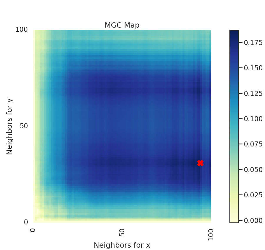
A unique property of MGC is a MGC map, which is a (n, n) map (or (n, k) where
k is less than n if there are repeated values). This shows you the test statistics
at all these different "scales". The optimal scale is an ordered pair that indicates
nearest neighbors where the test statistic is maximized and is marked by a red "X".
This optimal scale is the location of the test statistic.
The heat map gives insights into the nature of the dependency between x and y.
Otherwise, this test runs like any other test.
We can plot it below:
import matplotlib.pyplot as plt
import matplotlib.ticker as ticker
import seaborn as sns

# make plots look pretty
sns.set(color_codes=True, style="white", context="talk", font_scale=1)

mgc_map = mgc_dict["mgc_map"]
opt_scale = mgc_dict["opt_scale"]  # i.e. maximum smoothed test statistic
print("Optimal Scale:", opt_scale)

# create figure
fig, (ax, cax) = plt.subplots(
    ncols=2, figsize=(9, 8.5), gridspec_kw={"width_ratios": [1, 0.05]}
)

# draw heatmap and colorbar
ax = sns.heatmap(mgc_map, cmap="YlGnBu", ax=ax, cbar=False)
fig.colorbar(ax.get_children()[0], cax=cax, orientation="vertical")
ax.invert_yaxis()

# optimal scale
ax.scatter(opt_scale[1], opt_scale[0], marker="X", s=200, color="red")

# make plots look nice
ax.set_title("MGC Map")
ax.xaxis.set_major_locator(ticker.MultipleLocator(10))
ax.xaxis.set_major_formatter(ticker.ScalarFormatter())
ax.yaxis.set_major_locator(ticker.MultipleLocator(10))
ax.yaxis.set_major_formatter(ticker.ScalarFormatter())
ax.set_xlabel("Neighbors for x")
ax.set_ylabel("Neighbors for y")
ax.set_xticks([0, 50, 100])
ax.set_yticks([0, 50, 100])
ax.xaxis.set_tick_params()
ax.yaxis.set_tick_params()
cax.xaxis.set_tick_params()
cax.yaxis.set_tick_params()
plt.show()
Out:
Optimal Scale: [27, 99]
For linear data, we would expect the optimal scale to be at the maximum nearest neighbor pair. Since we consider nonlinear data, this is not the case.
Kernel mean embedding random forest (KMERF)
Random-forest based tests exploit the theoretical properties of decision tree based classifiers to create highly accurate tests (especially in cases of high dimensional data sets).
Kernel mean embedding random forest (KMERF) is one such test, which uses
similarity matrices as a result of random forest to generate a test statistic and
p-value. More details can be found in hyppo.independence.KMERF.
Note
- Pros
Highly accurate, powerful independence test for multivariate and nonlinear data
Gives information about releative dimension (or feature) importance
- Cons
Very slow (requires training a random forest for each permutation)
Unlike other tests, there is no compute_distance
parameter. Instead, the number of trees can be set explicitly, and the type of
classifier can be set ("classifier" in the case where the return value \(y\) is
categorical, and "regressor" when that is not the case). Check out
sklearn.ensemble.RandomForestClassifier and
sklearn.ensemble.RandomForestRegressor for additional parameters to change.
Otherwise, this test runs like any other test.
from hyppo.independence import KMERF
from hyppo.tools import cubic

# 100 samples, 5D sim
x, y = cubic(n=100, p=5)

# get the feature importances (only need the statistic)
_, _, kmerf_dict = KMERF(ntrees=5000).test(x, y, reps=0)
Because this test is random-forest based, we can get feature importances. This gives us relative importances value of dimension (i.e. feature). KMERF returns a normalized version of this parameter, and we can plot these importances:
importances = kmerf_dict["feat_importance"]
dims = range(1, 6)  # range of dimensions of simulation


import matplotlib.pyplot as plt
import seaborn as sns

# make plots look pretty
sns.set(color_codes=True, style="white", context="talk", font_scale=1)

# plot the feature importances
plt.figure(figsize=(9, 6.5))
plt.plot(dims, importances)
plt.xlim([1, 5])
plt.xticks([1, 2, 3, 4, 5])
plt.xlabel("Dimensions")
plt.ylim([0, 1])
plt.yticks([])
plt.ylabel("Normalized Feature Importance")
plt.title("Feature Importances")
plt.show()
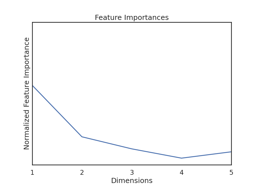
We see that feature importances decreases as dimension increases. This is true for
most of the simulations in hyppo.tools.
Maximal Margin Correlation
Maximial Margin Correlation takes the independence tests in
hyppo.independence, and compute the maximal correlation of pairwise comparisons
between each dimension of x and y.
More details can be found in hyppo.independence.MaxMargin.
Note
- Pros
As powerful as some of the tests within this module
Minimal decrease in testing power as dimension increases
- Cons
Adds computational complexity, so can be slow
These tests have an indep_test parameter corresponding to the desired independence
test to be run. All the parameters from the above tests can also be modified, and see
the relevant section of reference documentation in hyppo.independence for more
information.
These tests runs like any other test.
Friedman Rafsky Test for Randomness
This notebook will introduce the usage of the Friedman Rafsky test, a multivariate extension of the Wald-Wolfowitz runs test to test for randomness between two multivariate samples. More specifically, the function tests whether two multivariate samples were independently drawn from the same distribution.
The question proposed in 'Multivariate Generalizations of the Wald-Wolfowitz and Smirnov Two-Sample Tests' is that of how to extend the univariate Wald-Wolfowitz runs test to a multivariate setting.
The univariate Wald-Wolfowitz runs test is a non-parametric statistical test that checks a randomness hypothesis for a two-valued data sequence. More specifically, it can be used to test the hypothesis that the elements of a sequence are mutually independent. For a data sequence with identifiers of two groups, say: \(X , Y\) we begin by sorting the combined data set \(W\) in numerical ascending order. The number of runs is then defined by the number of maximal, non-empty segments of the sequence consisting of adjacent and equal elements. So if we designate every \(X = +, Y = -\) an example assortment of the 15 element long sequence of both sets could be given as \(+++----++---+++\) which contains 5 runs, 3 of which positive and 2 of which negative. By randomly permuting the labels of our data a large number of times, we can compare our true number of runs to that of the random permutations to determine the test statistic and p-value.
For extension to the multivariate case, we determine a neighbor not by proximity in numerical order, but instead by euclidean distance between each point. The data is then 'sorted' via a calculation of the minimum spanning tree in which each point is connected to each other point with edge weight equal to that of the euclidean distance between the two points. The number of runs is then determined by severing each edge of the MST for which the points connected do not belong to the same family. Similarly to the univariate case, the labels associated with each node are then permuted randomly a large number of times, we can compare our number of true runs to the random distribution of runs to determine the multivariate test statistic and p-value.
As such, we see that this set of data contains 3 such runs, and again by randomizing the labels of each data point we can determine the test statistic and p-value for the hypothesis that to determine the randomness of our combined sample. It's worth noting that X and Y need not have the same number of samples, just that they posess the same number of multivariate features. Lastly, labels for X and Y need not be 0 and 1, they just need be consistent across samples. These tests runs like any other test.
Test statistic range: \([2, m+n]\), where \(m\) and \(n\) are the number of samples in sets \(X\) and \(Y\) respectively.
Total running time of the script: ( 0 minutes 13.668 seconds)