Note
Click here to download the full example code
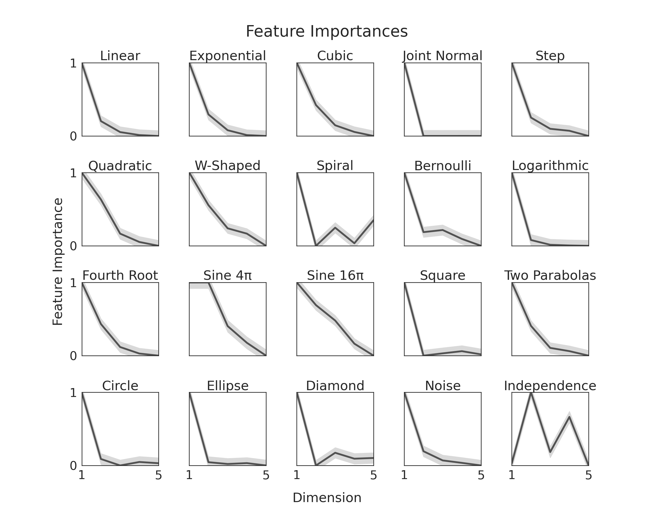
Feature Importances
hyppo.independence.KMERF class is a powerful
independence test built upon random forest and kernel embedding methods.
All random forests return feature importances, and since KMERF uses random forest as a
kernel, we can use feature importances to tell use which of our dimensions (or features)
contributes most to the decision of accepting or rejecting the null hypothesis. This
idea tremendously improves the interpretability of the tests.
Here, we will show you, given our simulations, which we modify such that y is one
dimensional and dimensions become less important as dimensionality increases. We do
this to verify that feature importance is being correctly measured. To see how we
modified the simulations, checkout this
notebook.
It is worth noting the last simulation does not follow this general trend. That is
because we each dimension in that one is equally important.
import os
import sys
import warnings

import matplotlib.pyplot as plt
import numpy as np
import seaborn as sns
from hyppo.independence import KMERF
from hyppo.tools import SIMULATIONS
from joblib import Parallel, delayed
from scipy.stats import norm

# add file path for precomputed data
sys.path.append(os.path.realpath(".."))

# make plots look pretty
sns.set(color_codes=True, style="white", context="talk", font_scale=2)

# constants
REPS = 100  # number of replications to average
DIM = 5  # 5D simulation
FOREST_SIZE = 5000  # size of forest
SIM_SIZE = 200  # size of simulation

# simulation titles
SIM_TITLES = [
    "Linear",
    "Exponential",
    "Cubic",
    "Joint Normal",
    "Step",
    "Quadratic",
    "W-Shaped",
    "Spiral",
    "Bernoulli",
    "Logarithmic",
    "Fourth Root",
    "Sine 4\u03C0",
    "Sine 16\u03C0",
    "Square",
    "Two Parabolas",
    "Circle",
    "Ellipse",
    "Diamond",
    "Noise",
    "Independence",
]


def tree_import(sim_name):
    """Train a random forest for a given simulation, calculate feature importance."""
    # simulate data
    x, y = SIMULATIONS[sim_name](SIM_SIZE, DIM)
    if y.shape[1] == 1:
        y = y.ravel()

    with warnings.catch_warnings():
        # get feature importances
        _, _, importances = KMERF(forest="regressor", ntrees=FOREST_SIZE).test(
            x, y, reps=0
        )

    return importances


def estimate_featimport(sim_name, rep):
    """Run this function to calculate the feature importances"""
    est_featimpt = tree_import(sim_name)
    np.savetxt(
        "../examples/data/{}_{}.csv".format(sim_name, rep), est_featimpt, delimiter=","
    )

    return est_featimpt


# At this point, we would run this bit of code to generate the data for the figure and
# store it under the "data" directory. Since this code takes a very long time, we have
# commented out these lines of codes. If you would like to generate the data, uncomment
# these lines and run the file.
#
# outputs = Parallel(n_jobs=-1, verbose=100)(
#     [
#         delayed(estimate_featimport)(sim_name, rep)
#         for sim_name in SIMULATIONS.keys()
#         for rep in range(REPS)
#     ]
# )


def plot_featimport_confint():
    """Plot feature importances and 95% confidence intervals"""
    fig, ax = plt.subplots(nrows=4, ncols=5, figsize=(25, 20))

    plt.suptitle("Feature Importances", y=0.93, va="baseline")

    for i, row in enumerate(ax):
        for j, col in enumerate(row):

            # get the panel location and simulation name
            count = 5 * i + j
            sim_name = list(SIMULATIONS.keys())[count]

            # extract data from the CSV file and store the data in an array
            all_impt = np.zeros((REPS, DIM))
            for rep in range(REPS):
                forest_impt = np.genfromtxt(
                    "../examples/data/{}_{}.csv".format(sim_name, rep), delimiter=","
                )
                all_impt[rep, :] = forest_impt

            # get the mean importances for the simulation, also calculate 95% CI
            # interval
            mean_impt = np.mean(all_impt, axis=0)
            mean_impt -= np.min(mean_impt)
            mean_impt /= np.max(mean_impt)
            low, high = norm.interval(
                0.95, loc=mean_impt, scale=np.std(mean_impt, axis=0) / np.sqrt(REPS)
            )

            # plot the figure lines, and the 95% CI
            col.plot(
                range(1, DIM + 1),
                mean_impt,
                color="#525252",
                lw=5,
                label="Averaged Data",
            )
            col.fill_between(range(1, DIM + 1), low, high, color="#d9d9d9")

            # make the data look pretty for each pannel
            col.set_xticks([])
            if i == 3:
                col.set_xticks([1, 5])
            col.set_xlim([1, 5])
            col.set_ylim([0, 1])
            col.set_yticks([])
            if j == 0:
                col.set_yticks([0, 1])
            col.set_ylabel("")
            col.set_xlabel("")
            col.set_title(SIM_TITLES[count])

    # misc entire plot
    fig.text(0.5, 0.04, "Dimension", ha="center")
    fig.text(0.08, 0.5, "Feature Importance", va="center", rotation="vertical")
    plt.subplots_adjust(hspace=0.50, wspace=0.40)


# plot the feature importances
plot_featimport_confint()
Total running time of the script: ( 0 minutes 0.858 seconds)